Method

Methods

Here we describe how to reconstruct the fibers of SLF and derive a lateralization score for each subject. We will then relate the lateralization score to gender and handedness through a two-way ANOVA model.

The steps include: For each subject, on the native subject space

1. FOD estimation: Obtain the BJS FOD estimator for each voxel within the probabilistic SLF masks;
2. Peak detection: Identify peak(s) of the estimated FODs;
3. Tractography: Apply the DiST tracking algorithm using the probabilistic SLF masks as both the seeding mask and the terminating mask;
4. Streamline selection: Select streamlines from the tractographic reconstructed tracks that are passing through the binary SLF masks at both ends;
5. Feature extraction: Define a lateralization score as the (relative) difference between the numbers of (selected) streamlines of the left- and right- hemisphere SLF.

Moreover, both FOD estimation and tractography are confined within the white matter voxels (obtained through the white matter segmentation preprocessing step).

Section 4.1: FOD Estimation and Peak Detection

These steps take ~ 20 minutes per 100k voxels.

For each subject, we estimated FOD for voxels within the probabilistic SLF masks (from Step 4 of the preprocessing) on the native subject space. We then identified the peak(s) of the estimated FODs by a peak detection algorithm (Yan et al., 2018). Moreover, non-white matter voxels within these masks are automatically specified as being isotropic and thus has no direction. The peak detection step associates each voxel with either none, one or multiple direction(s) and its results will be used as inputs for the DiST tracking algorithm.

Section 4:2: Tractography

This step takes ~ 1h for a 40k ROI.

Here we applied the DiST tracking algorithm (Wong et al., 2016) which is a deterministic tractography algorithm and can handle zero or multiple directions within one voxel and thus is suitable for crossing fiber regions. Moreover, we used the probabilistic masks for SLF (one on each hemisphere) from the JHU White-Matter Tractography Atlas as both the seeding mask and the terminating mask, meaning that tracking starts from every (white-matter) voxel within these masks and trajectories will be terminated while leaving the SLF region specified by these masks. Another stopping criterion we used is when there is no viable voxels within two steps, where non-viable voxels are those leading to trajectory bending more than 60 degrees or being isotropic (e.g., a non-white matter voxel).

The above regional-seeding approach is suitable for extracting a specific pathway (here SLF) or mapping tracts from a specific region. One advantage of the regional-seeding approach to the whole-brain-seeding approach is that the former is computationally much less intensive and scales better to processing large number of subjects/images. The regional-seeding approach may also take advantage of existing knowledge in brain anatomy. A potential disadvantage of a regional-seeding approach is to have incomplete track reconstruction. This can be mitigated by using anatomically informed masks such as those from a white matter atlas as we have done here.

Section 4.3: Streamline Selection

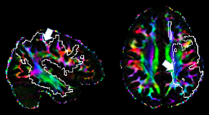
One common criterion for streamline selection is to only retain tracks longer than a certain length (a commonly used threshold is 10mm). The rationale is that shorter tracks are unreliable. Moreover, as can be seen from the orientation color map below, the SLF region crosses with the corticospinal tract (indicated by blue-color). As a result, the reconstructed fibers contain not only those of SLF, but also some of CST.

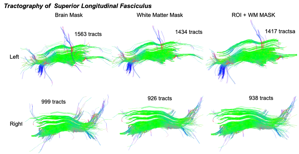
To better dissect SLF from the initial tractography results, we used binary masks from AutoPtx to conduct streamline selection where only tracks (streamlines) that pass through AutoPtx binary masks at both ends are retained. The plot below shows SLF reconstruction (after streamline selection) of one HCP subject, using whole-brain-seeding (left panel), whole-brain-seeding with the white matter mask (middle panel) and regional-seeding with the white matter mask (right panel). As can be seen there, the tractography results are visually similar and regional-seeding does not lose too many tracks.

Section 4.4: Feature Extraction

After tractography and streamline selection, various brain structural connectivity related features can be extracted including the number of streamlines, the lengths of streamlines, etc. Here we focused on the difference between the left- and right- hemisphere SLF for the purpose of investigating potential lateralization of SLF and its association with gender and handedness.

For each subject, we calculate a lateralization score (LS) based on the relative difference between the numbers of selected streamlines from the left- and right- hemisphere SLF, respectively:

\[LS=\frac{\mbox{Streamlines in Left SLF} - \mbox{Streamlines in Right SLF}}{(\mbox{Streamlines in Left SLF} + \mbox{Streamlines in Right SLF})/2}\]

Here, the denominator serves the purpose of normalization so that the LS from subjects with different brain sizes are comparable. As can be seen from the plot in Section 5.2, the LS is uncorrelated with the (relative) difference between the numbers of voxels in the left- and right- hemisphere SLF masks. A similar score was used by Catani et al 2007 for studying lateralization of the language pathway.