HCP dMRI data preprocessing

This section describes how to download and process diffussion MRI (dMRI) data from the Human Connectome Project (HCP) database using various neuroconductor R packages (https://neuroconductor.org/)

HCP D-MRI Data Preprocessing

This section describes how to process D-MRI data from the Human Connectome Project (HCP) database. We use FSL, a library of tools for MRI, fMRI and D-MRI imaging data, as well as its R wrapper, the fslr R package from neuroconductor. Both FSL and fslr need to be installed.

library(fslr)

Notes: Processing time is measured under a Xeon 72 core, 2.3GHz, 256GB RAM linux server.

Step 0 – HCP Preprocessing Pipeline

D-MRI data from HCP database have already been (minimally) processed. The detailed information about the HCP minimal preprocessing pipeline can be found in Glasser et al. 2013 and on page 133 of the HCP reference manual. The scripts are available at HCPpipelines git repository.

These steps include:

1. Intensity normalization
2. EPI distortion correction (TOPUP algorithm in FSL)
3. Eddy current correction (EDDY algorithm in FSL)
4. Gradient nonlinearity correction
5. Registration (6 DOF rigid body) of the mean b0 image (T2-weighted image) to native volume T1-weighted image by FSL FLIRT BBR and FreeSurfer bbregister algorithms; and the transformation of diffusion data, gradient deviation, and gradient directions to the 1.25mm structural space (T1w space). Moreover, (T1w co-registered) T2w extracted brain mask ‘nodif_brain_mask.nii.gz’ by FSL BET algorithm is also provided.

Thus, the HCP D-MRI data have already been co-registered to the structural (T1w) space. In the following, we are going to focus on segmentation based on T1 weighted image and registration of T1 weighted image onto the standard space (MNI152_T1) through FSL FAST segmentation algorithm and FLIRT/FNIRT registration algorithms, respectively.

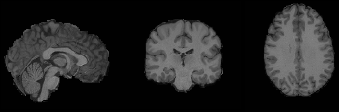
Step 1 – T1w Brain Extraction

This step takes a few seconds per image.

The original T1w and D-MRI images contain both skull and the brain. The BET (Smith 2002) algorithm in FSL can be used to extract brain from original images, which deletes non-brain tissues from an image of the whole head. In particular, extracted T1w images are needed for segmentation and registration. We use the (co-registered) T2w extracted brain mask provided by HCP preprocessing pipeline (‘nodif_brain_mask.nii.gz’) and apply that to the T1 image to create a T1w extracted brain. The rationale to use T2w extracted brain mask is because T2w image provides better contrasts between brain tissues and non-brain tissues.

Apply T2w extracted brain mask to T1w

Here we use the fslmaths tool to multiply a binary mask (the T2w extracted brain mask ‘nodif_brain_mask.nii.gz’) with an image (the original T1w image ‘T1w_acpc_dc_restore_1.25.nii.gz’).

The following is the shell code:

fslmaths "/user_path/T1w_acpc_dc_restore_1.25.nii.gz" -mul
"/user_path/nodif_brain_mask.nii.gz"
"/user_path/T1w_acpc_dc_restore_1.25_brain.nii.gz"

The following is the corresponding R wrapper function:

bet_w_fslmaths<-function(T1w, mask, outfile, intern=FALSE, verbose=TRUE, retimg=T, ...){
  cmd <- get.fsl()
  if (retimg) {
    if (is.null(outfile)) {
      outfile = tempfile()
    }
  } else {
    stopifnot(!is.null(outfile))
  }
  T1w = checkimg(T1w, ...)
  mask = checkimg(mask, ...)
  outfile = checkimg(outfile, ...)
  outfile = nii.stub(outfile)
  cmd <- paste0(cmd, sprintf("fslmaths \"%s\" -mul \"%s\"  \"%s\"", 
                             T1w, mask, outfile))
  if (verbose) {
    message(cmd, "\n")
  }
  res = system(cmd, intern = intern)
  ext = get.imgext()
  outfile = paste0(outfile, ext)
  return(res)
}

Usage:

bet_w_fslmaths(T1w = paste0(user_path,'T1w_acpc_dc_restore_1.25.nii.gz'),
               mask = paste0(user_path,'nodif_brain_mask.nii.gz'), 
               outfile = paste0(user_path,'T1w_acpc_dc_restore_1.25_brain.nii.gz'))

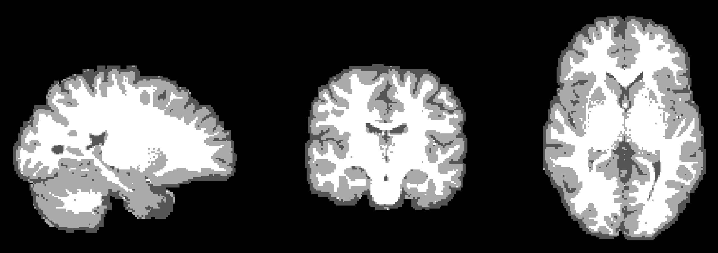
Step 2 – White Matter Segmentation

This step takes ~ 4 minutes per image.

FAST segmentation: The FAST algorithm (Zhang et al. 2001) classifies each voxel in the brain into different tissue types (e.g. CSF – cerebrospinal fluid, GM – grey matter, WM – white matter) from various image sources (e.g., T1w, T2w). Since T1w images provide better contrasts between white matter and grey matter, we apply FAST to the T1w extracted brain (‘T1w_acpc_dc_restore_1.25_brain.nii.gz’) from Step 1.

fast(file = paste0(user_path,'T1w_acpc_dc_restore_1.25_brain.nii.gz'), 
     outfile = nii.stub(paste0(user_path,'T1w_acpc_dc_restore_1.25_brain.nii.gz')), 
     opts = '-N')

*Outputs from *FAST **:

• ‘T1w_acpc_dc_restore_1.25_brain_seg.nii.gz’: binary segmentation (all classes in one image): e.g. 1 – CSF, 2 – GM, 3 –WM if the input is T1w image with 3 classes.

• ‘T1w_acpc_dc_restore_1.25_brain_pve.nii.gz’: one partial volume image for each class (pve0 – CSF, pve1 – GM, pve2 – WM, if the input is T1w image with 3 classes). Each voxel has a value between 0 and 1 representing the proportion of tissue in the corresponding class.

White matter mask is created by binarising the white matter partial volume image (‘T1w_acpc_dc_restore_1.25_brain_pve2.nii.gz’) where voxels with positive white matter partial volume are included in the white matter mask.

Step 3 – Subject to Standard Space Registration

In this step, the T1w image is registered to a standard space (here the T1-weighted MNI template MNI152_T1). We will apply linear registration by the FLIRT algorithm to register T1w to MNI152_T1, followed by the nonlinear registration by the FNIRT algorithm. Both brain extracted and non-extracted MNI152 template images are provided in the folder ‘/usr/local/fsl/data/standard/’.

Step 3.1 FLIRT:

This step takes ~10 seconds per image.

The linear registration tool FLIRT in FSL can perform both intra- (6 DOF) and inter-modal (12 DOF) brain image intensity-based registration. FLIRT takes extracted brain images as input and reference, respectively.

flirt(infile = paste0(user_path,'T1w_acpc_dc_restore_1.25_brain.nii.gz'),
      reffile = '/usr/local/fsl/data/standard/MNI152_T1_2mm_brain.nii.gz',
      omat = paste0(user_path,'org2std.mat'),
      dof = 12,
      outfile = paste0(user_path,'T1w_acpc_dc_restore_1.25_brain_flirt12.nii.gz'))

Step 3.2 FNIRT:

This step takes ~ 4.5 minutes per image.

The nonlinear registration tool FNIRT in FSL can only register images of the same modality. Hence we will need to first register the T1w image to the T1w MNI template (MNI152_T1). We also need to initialize the nonlinear registration by a linear (12 DOF) registration to get the orientation and size of the image close enough for the nonlinear registration. Therefore, we need to first run the linear registration tool FLIRT. Moreover, FNIRT uses the original image instead of the brain extracted version for both input and reference, so that any errors in brain extraction do not influence the local registration.

Specifically, FNIRT takes the transformation matrix (‘org2std.mat’ specified in ‘–aff’) from FLIRT output (Step 3.1: affine transformation with 12 DOF), the original T1w image, and non brain extracted (i.e., with skull) MNI152_T1 template.

opt_fnirt=paste0(' --aff=', user_path, 'org2std.mat',  
                 ' --config=/usr/local/fsl/etc/flirtsch/T1_2_MNI152_2mm.cnf',
                 ' --cout=', user_path, 'org2std_coef.nii.gz',  
                 ' --fout=', user_path, 'org2std_warp.nii.gz')  

fnirt(infile = paste0(user_path, 'T1w_acpc_dc_restore_1.25.nii.gz'),
      reffile = "/usr/local/fsl/data/standard/MNI152_T1_2mm.nii.gz",
      outfile = paste0(user_path, 'T1w_acpc_dc_restore_1.25_fnirt.nii.gz'),
      opts = opt_fnirt)

Outputs from FNIRT:

• ‘T1w_acpc_dc_restore_1.25_fnirt.nii.gz’: the transformed image.

• –cout ‘org2std_coef.nii.gz’: the spline coefficient and a copy of the affine transform.

• –fout ‘org2std_warp.nii.gz’: actual warp-field in the x,y,z directions.

Step 4 – From Standard Space to Native Space

In Step 3, we conduct registration which transforms an image to a standard template space. Here, we derive the inverse transformation from a standard space to a native space. This is useful for moving masks from a standard space template to the native space. We will use the invwarp and applywarp functions in FSL.

Step 4.1 Invert a transformation by invwarp

This step takes ~ 1 minute per image.

Suppose we want to invert the warp-field (‘org2std_warp.nii.gz’) from the FNIRT registration output. Then the original T1w image ‘T1w_acpc_dc_restore_1.25.nii.gz’ is used as reference and the output is stored in ‘std2org_warp.nii.gz’. The following is the shell code:

invwarp(reffile=paste0(user_path,'T1w_acpc_dc_restore_1.25.nii.gz'),
        infile=paste0(user_path,'org2std_warp.nii.gz'),
        outfile=paste0(user_path,'std2org_warp.nii.gz'))

The following is the corresponding R wrapper function:

invwarp<-function (reffile, infile, outfile, intern=FALSE, opts='', verbose=TRUE, retimg=T, ...) 
{
  cmd <- get.fsl()
  if (retimg) {
    if (is.null(outfile)) {
      outfile = tempfile()
    }
  }
  else {
    stopifnot(!is.null(outfile))
  }
  infile = checkimg(infile, ...)
  reffile = checkimg(reffile, ...)
  outfile = checkimg(outfile, ...)
  outfile = nii.stub(outfile)
  cmd <- paste0(cmd, sprintf("invwarp --ref=\"%s\" --warp=\"%s\" --out=\"%s\" %s", 
                             reffile, infile, outfile, opts))
  if (verbose) {
    message(cmd, "\n")
  }
  res = system(cmd, intern = intern)
  ext = get.imgext()
  outfile = paste0(outfile, ext)
  
  return(res)
}

Step 4.2: Apply a transformation to an image by applywarp

This step takes ~ 10 seconds per image.

Suppose we want to move a mask on a template space to the native space. The following is the shell code:

fsl_applywarp(infile = paste0(user_path,'mask_on_template.nii.gz'),
              reffile = paste0(user_path,'T1w_acpc_dc_restore_1.25.nii.gz') ,
              outfile = paste0(user_path,'mask_on_original_space.nii.gz'),
              warpfile = paste0(user_path,'std2org_warp.nii.gz'))

In the following, we first chose the Superior Longitudinal Fasciculus (SLF) masks (probabilistic masks on two hemispheres: SLF_L – 41694 voxels, SLF_R – 38386 voxels; brighter color corresponds to higher probability of being on SLF) according to the JHU White-Matter Tractography Atlas (Wakana et al. 2007, Hua et al. 2008) on the MNI152_T1_2mm template space (left panel) using FSLeyes. We then mapped these masks back to the native T1w space of one HCP subject (right panel) using the applywarp function. We will later use these masks as both seeding and terminating masks in the DiST tractography algorithm for SLF reconstruction (Section 4). Moreover, binary masks (1 – white color) from AutoPtx will be used for further streamline selection of the tractography results to better dissect SLF (Section 4). The binary masks are situated at the margins of the portion of the probabilistic masks where the probability of being on SLF is high (indicated by bright color).

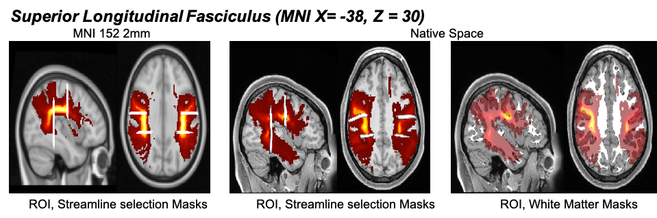
Using FSLeyes and FSL atlases and templates to create masks is illustrated in the Appendix A.1.